The Universal Sentence Encoder and Locality Sensitive Hashing..
improving search time and file size for sentence embedding searches
(Yet another way to browse Sailor Moon)

the universal sentence encoder
The Universal Sentence Encoder is a model trained on a variety of language data sources. It is able to turn a sentence into a 512-dimension vector (also called an embedding). The goal is to have semantically similar sentences produce vectors that point in a similar direction.
Embeddings are a common way for neural nets to represent real higher dimension data and are especially common in language processing. Consider how many possible word combinations there are in sentences, and the variety of sentence lengths. It's hard to compare this information programmatically. Making embeddings especially useful.
So a sentence is fed into the network and an array of 512 numbers is produced, which can be compared to other arrays created from other sentences. These embeddings can be used for a variety of natural language processing tasks, but in this case to compare sentence similarity.
The neural network is capable of doing this as it was trained on sentence
pairs that had their semantic textual similarity scored by humans.
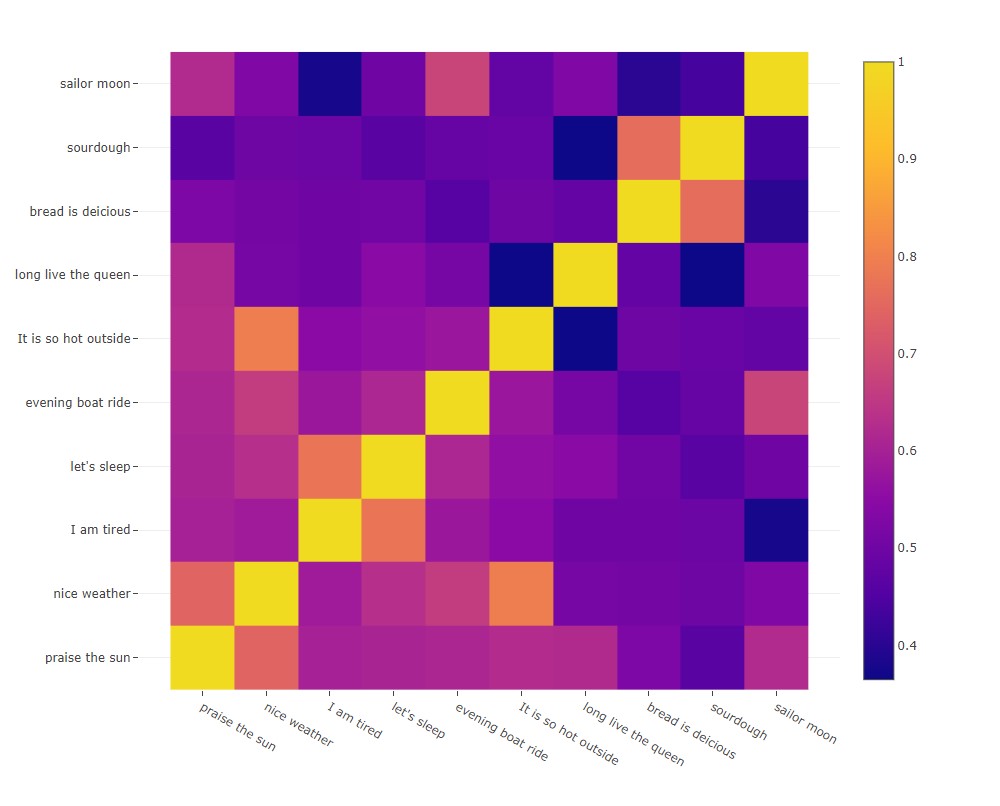
Let's see how some sentences compare for fun.
The image below shows several sentences compared to each other and scored based on their
semantic similarity using the universal sentence encoder model.
 Create your
own heatmap here
Create your
own heatmap here
Comparing Embeddings
Let's take a look at an example embedding, this one is for the sentence, "praise the sun"
[ -0.01643446274101734, -0.047866735607385635, 0.01116135623306036, -0.032162975519895554, -0.04119051992893219, -0.049514010548591614, 0.05056055262684822, 0.01861172914505005, 0.02079540677368641, 0.03788421303033829, 0.055882297456264496, 0.052787601947784424, -0.04854540899395943, 0.0047414726577699184, -0.053531713783741, -0.017291227355599403, 0.053345393389463425, 0.05225902795791626, 0.044134367257356644, 0.034594688564538956, 0.02990477718412876, 0.01906985603272915, 0.04899447783827782, 0.055814746767282486, -0.05602262541651726, 0.05459308251738548, 0.05091241002082825, -0.05024508386850357, -0.05322225019335747, 0.020622193813323975, 0.022310415282845497, -0.05342493951320648, -0.03910081088542938, -0.054072655737400055, 0.04943077266216278, -0.05404074117541313, -0.05312085151672363, 0.048237964510917664, 0.052785295993089676, -0.04522813856601715, 0.053926967084407806, 0.03370456025004387, 0.05236560106277466, 0.0015304642729461193, -0.044569939374923706, -0.04093872010707855, 0.0400158166885376, 0.05586504936218262, 0.040547121316194534, 0.0036303112283349037, 0.05467100441455841, -0.05315506085753441, 0.05460590869188309, -0.05341360718011856, 0.019216563552618027, 0.014945510774850845, 0.008523264899849892, -0.05486554652452469, -0.05196134373545647, -0.0503271222114563, -0.054707158356904984, -0.03312518447637558, -0.05008922889828682, 0.0006174301961436868, -0.03885316103696823, 0.05602826178073883, -0.05558229237794876, -0.03280400112271309, 0.0557483471930027, -0.020747335627675056, -0.04034963250160217, -0.05323438718914986, 0.05147049203515053, 0.05478457361459732, 0.050157900899648666, -0.05495397374033928, 0.040603939443826675, 0.056042611598968506, 0.043434031307697296, -0.0055681923404335976, -0.03814433142542839, -0.03673834726214409, -0.05543023720383644, -0.05131136626005173, -0.05583127215504646, 0.04594847932457924, 0.05276202782988548, -0.05573916807770729, -0.022053785622119904, 0.0015039695426821709, -0.0377194806933403, 0.023686300963163376, -0.04683661460876465, 0.04619279131293297, -0.04374907910823822, -0.027344444766640663, 0.038678839802742004, -0.020303141325712204, 0.051446061581373215, -0.021707113832235336, -0.05371095985174179, 0.055392805486917496, 0.05516625568270683, 0.056031569838523865, -0.046048443764448166, -0.052267421036958694, 0.036351095885038376, 0.042035214602947235, -0.030406028032302856, -0.027976704761385918, -0.024354681372642517, -0.03456025943160057, -0.048526324331760406, -0.054300062358379364, 0.03975285217165947, 0.03405265137553215, -0.0008716466836631298, 0.04143061488866806, -0.017759624868631363, 0.04933466389775276, 0.04317356273531914, -0.05370345711708069, 0.046637848019599915, -0.05604122579097748, -0.04903582111001015, -0.008755053393542767, 0.02665846049785614, 0.05143268033862114, 0.015641331672668457, 0.053754791617393494, 0.03222831338644028, -0.05548969656229019, -0.05565796047449112, 0.05579647049307823, -0.025518905371427536, -0.05387597158551216, 0.02367117628455162, 0.043358735740184784, -0.032881706953048706, 0.04977487027645111, -0.025500651448965073, -0.01830417476594448, 0.054875925183296204, 0.05603192746639252, -0.0505065955221653, -0.023587802425026894, 0.028091568499803543, -0.05503155291080475, 0.03317264840006828, -0.05222945660352707, 0.0002477589878253639, -0.05411040037870407, -0.04951809346675873, -0.003709644079208374, 0.05603909492492676, 0.00677878875285387, 0.03319043666124344, -0.052565574645996094, -0.05374324321746826, 0.05126998946070671, -0.010412076488137245, -0.016527077183127403, 0.055314358323812485, -0.05408173426985741, 0.008594626560807228, 0.055709823966026306, 0.013491012156009674, -0.0006980478647165, 0.0053011467680335045, 0.045773740857839584, -0.05204932764172554, -0.023253854364156723, -0.05288105458021164, 0.045529551804065704, -0.055810973048210144, 0.006248749326914549, -0.052872903645038605, 0.012982008047401905, 0.04929075390100479, 0.051177412271499634, 0.024482639506459236, -0.0023270556703209877, 0.05582268536090851, -0.05187274515628815, 0.05578025430440903, -0.02887865900993347, -0.055860910564661026, 0.049252405762672424, 0.027567410841584206, 0.004360144957900047, -0.03805725648999214, 0.04781678318977356, 0.02349051833152771, -0.05355745181441307, -0.0010168420849367976, 0.019375935196876526, -0.048489831387996674, 0.05290268734097481, -0.0514141209423542, -0.05219649523496628, 0.053786858916282654, 0.04703744500875473, -0.05548414960503578, -0.05426885187625885, 0.04358344152569771, -0.04335813596844673, 0.055667418986558914, -0.05191067233681679, 0.050331346690654755, 0.052997346967458725, -0.05290118604898453, 0.05595087260007858, 0.02919776737689972, 0.0279071107506752, -0.05300073325634003, -0.025899618864059448, 0.05566255375742912, 0.01740713231265545, 0.05597109720110893, 0.05386003479361534, 0.04719238728284836, -0.0413287952542305, 0.05515514686703682, -0.05304962396621704, -0.0282291192561388, -0.016887780278921127, -0.02695431374013424, 0.018786640837788582, 0.05564965307712555, -0.05578072369098663, 0.02692331001162529, 0.042407725006341934, -0.05515687167644501, 0.05270160362124443, -0.011442351154983044, 0.055934712290763855, 0.05354756489396095, 0.03316701203584671, 0.05588717758655548, 0.05604216828942299, -0.008422136306762695, 0.043577276170253754, -0.008080055005848408, 0.016125492751598358, 0.046945225447416306, 0.043736327439546585, -0.023303015157580376, -0.050779227167367935, 0.04854461923241615, -0.0560176819562912, -0.04963786527514458, -0.054972484707832336, 0.051782578229904175, -0.05325941741466522, 0.01675291731953621, 0.05401768162846565, -0.029279962182044983, 0.029603365808725357, 0.05384274199604988, 0.05026647076010704, -0.05591430142521858, 0.014729233458638191, 0.004318914841860533, 0.04583499953150749, -0.028199832886457443, 0.05517265945672989, 0.05195918306708336, 0.03361981362104416, -0.005860268138349056, 0.054360758513212204, -0.04790390655398369, -0.04412402957677841, 0.05526090785861015, -0.04397204518318176, 0.0510873906314373, 0.054974354803562164, -0.05430081859230995, 0.0511348582804203, -0.05075996369123459, -0.017456840723752975, -0.054586976766586304, 0.04988223314285278, -0.031048662960529327, -0.0019140191143378615, -0.00025244030985049903, -0.03073504939675331, -0.008409513160586357, 0.04650219529867172, 0.0459686703979969, -0.018416931852698326, -0.05508637800812721, 0.05005917325615883, -0.03366953879594803, -0.02187909558415413, 0.041992828249931335, -0.05555545166134834, 0.05599233880639076, 0.03982987254858017, 0.04466022178530693, 0.04570598155260086, 0.055467091500759125, 0.05319790542125702, -0.05507420003414154, 0.055999744683504105, -0.041691623628139496, -0.01942344382405281, -0.018287384882569313, 0.05570831894874573, -0.028560396283864975, -0.052859265357255936, 0.02748016081750393, -0.05497709661722183, 0.05500137433409691, 0.0538204200565815, 0.05325619876384735, -0.05123851075768471, -0.05441600829362869, -0.04787558317184448, 0.05543545261025429, 0.04792202636599541, 0.04059022665023804, -0.047015149146318436, 0.01801333576440811, -0.04497704282402992, 0.05537839233875275, -0.04872656241059303, -0.0498863160610199, -0.05248422548174858, 0.004491743631660938, -0.056007225066423416, 0.04945643991231918, -0.05558210611343384, -0.053780682384967804, 0.036105845123529434, 0.05598032474517822, 0.053630754351615906, -0.04550294950604439, 0.05588221922516823, -0.03173701465129852, 0.026102842763066292, -0.032342758029699326, 0.054514095187187195, 0.05471456050872803, 0.0535542294383049, 0.024944543838500977, 0.022099237889051437, 0.05573274940252304, 0.03772395849227905, -0.006928583141416311, 0.055451977998018265, 0.05255221948027611, -0.020383965224027634, 0.014840695075690746, -0.052972737699747086, 0.04729835316538811, 0.041253626346588135, -0.04857562109827995, -0.03430145978927612, 0.030324283987283707, 0.051337189972400665, 0.05483871325850487, 0.05280350521206856, -0.024308906868100166, -0.055778954178094864, -0.027072394266724586, -0.04774164780974388, 0.055680446326732635, -0.022918766364455223, -0.031212477013468742, -0.055910054594278336, -0.022955654188990593, -0.0385383665561676, 0.04803907498717308, -0.050335753709077835, 0.0509420782327652, 0.05588535591959953, -0.007357464637607336, 0.052812933921813965, 0.022859547287225723, 0.05572576820850372, -0.003088396741077304, 0.03805335611104965, -0.05365729704499245, 0.05554977431893349, 0.00746613135561347, -0.05584201589226723, 0.05582189932465553, -0.008294692263007164, -0.041224587708711624, -0.03395610302686691, -0.03327474743127823, -0.03447003290057182, 0.023300718516111374, 0.03380630537867546, 0.03800996020436287, 0.05538610741496086, 0.05519676208496094, -0.056026309728622437, -0.055212780833244324, 0.05570850148797035, 0.029411407187581062, 0.055867381393909454, -0.041572559624910355, 0.054851919412612915, -0.04785359278321266, -0.041999075561761856, 0.042050108313560486, -0.023656176403164864, 0.01810332201421261, -0.028811370953917503, -0.04434119910001755, -0.022894995287060738, -0.04691595211625099, 0.028853129595518112, 0.05067988112568855, -0.05385778471827507, -0.05336437001824379, -0.028338856995105743, 0.055960699915885925, 0.0556451715528965, 0.053908269852399826, -0.05120284855365753, -0.03537750989198685, -0.055464960634708405, -0.056009646505117416, -0.048401106148958206, 0.0520816408097744, 0.05341281741857529, 0.042371753603219986, -0.05149541050195694, 0.02432170696556568, -0.05589159578084946, -0.0253126323223114, -0.055962808430194855, 0.05288317799568176, -0.055515848100185394, -0.04950021579861641, 0.053132157772779465, 0.05560009181499481, -0.05382295697927475, 0.03887653723359108, 0.05554954335093498, 0.046343084424734116, 0.05601463466882706, -0.046690721064805984, 0.05519827827811241, 0.05464799702167511, -0.054447636008262634, 0.05284092575311661, 0.054841265082359314, 0.03104795143008232, -0.055980488657951355, 0.054428581148386, -0.02225598320364952, -0.04590776562690735, -0.0538906455039978, 0.018541937693953514, -0.05409042909741402, -0.008213928900659084, 0.048824261873960495, 0.04403650760650635, -0.05584526062011719, -0.0467953197658062, 0.023316213861107826, 0.0553462840616703, 0.05479169264435768, -0.03851236775517464, 0.0545991025865078, -0.050144799053668976, -0.052886318415403366, 0.05447651073336601, 0.04183284565806389, 0.03253893554210663, 0.04657915607094765, -0.046109311282634735, 0.05548405647277832, 0.05580862984061241, 0.03811436891555786, -0.05542745813727379, 0.03589120879769325, 0.00815376453101635, -0.055900316685438156, -0.05602550506591797, -0.006971255410462618, -0.05076229199767113, 0.05467640981078148, 0.0029950763564556837, 0.04073617234826088, -0.05401226133108139, 0.011864435859024525, -0.010817749425768852, 0.04748326912522316, -0.007380371447652578, 0.04826263338327408, 0.05093942582607269, 0.004084303975105286, 0.05559725686907768, 0.016932904720306396, 0.025586623698472977, 0.05064704641699791, -0.047627706080675125, 0.020730800926685333, -0.05533415824174881, 0.052814748138189316, -0.04870741814374924, -0.05315487086772919, 0.05516745150089264, 0.012046034447848797, -0.040742047131061554, -0.056016404181718826, 0.04769644886255264, 0.05575522035360336]
This array is a bit daunting to look at, and tbh could probably be rounded to fewer decimal places,
so for our visualizations, let's start with an array that has a
length of 2 and not 512, much easier to plot on a chart.
Check out the point below with x and y as our two dimensions, but we aren't thinking of this array
so
much as
a
point, but as more of a vector, with its direction and magnitude being its length from 0 and
the angle it forms, click the button to visualize as a vector lol
All graphs created using jsxGraph which is honestly worth a write up of its own
Let's call our vector a, the length or magnitude of a would be √(a₁² + a₂²), or
to consider it
in 2d space √(ax² + ay²), this is also
denoted as
|a|
An example in 2D space is much easier to visualize than 512D which our embeddings are in,
but is very useful as the math remains the same at higher
dimensions. If a was a 512-dimensional vector the value of |a| would be √(a₁² +
a₂² + a₃² + ...
a₅₁₂²)
The universal sentence encoder model was trained to have semantically similar sentences produce
embeddings
that have high angular similarity (the angle between them is
small/they point in the same direction).
Take a look at the 3 vectors below.
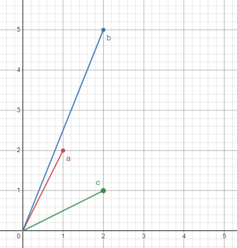 The euclidian distance between then ends of a and c is smaller, but we are comparing
the angle
between them as vectors, so a and b would be more similar than a and
c.
The euclidian distance between then ends of a and c is smaller, but we are comparing
the angle
between them as vectors, so a and b would be more similar than a and
c.
It can be costly to compute the angular similarity between embeddings
so it is more common to calculate their cosine similarity,
which is the same as the cosθ
of the angle between them.
Like angular similarity, if two vectors have a high cosine
similarity they will be pointing in a similar direction.
If you're like me and forget all basic trigonometry every few years, cosθ = adj/hyp for a
right-angle triangle.
And acos or on your calculators usually cos⁻¹ is the magic function we run cosθ
through
to get an angle.
That acos function is the part that is costly to compute
so it is what we will skip when checking only cosine similarity
Take a look below at how cosθ or the cosine similarity compares to the actual angle between two
vectors.
Drag the points around and see how the values change.
So we can see that cosθ will range from 1 when the angle is 0 (high cosine and angular
similarity)
to -1 when the angle is 180 (low cosine and angular similarity).
This can be sen in a plot of the cosine function.
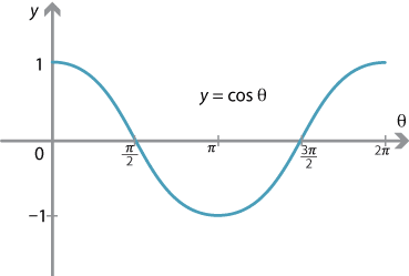
However cosθ doesn't scale linearly with the angular distance so it is not a good measure of
the
strength of the association between two vectors but it works just
as well for proportional association (seeing how close vectors are
compared to other vectors)
Now let's take a look at two vectors again, but we will lock one to 0° and change its
magnitude to consistently create a
right-angle triangle to show how we could calculate cosθ between them.
Of course it would be very easy to find the cosine similarity between vectors if they each formed
a nice right angle triangle with each other, one vector would be the adjacent and the other the
hypotenuse,
but sadly this isn't the case, like in the first example the vectors could have any magnitude and
we need a way to find the cosine similarity between vectors
regardless of their magnitudes, consider the image below. To find cosθ we need to
find the adjacent and hypotenuse of a right-angle triangle formed by our angle.
In this image the hypotenuse is easy to find, it is |a|, but we need to find L given only the
information for a and b.
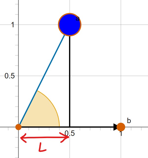
Here is an example where both vectors can be moved
Fortunately, there is a formula that allows us to find cosθ and by that also find L
using something called the dot product.
If we have two vectors of length 512, lets call them a and b again.
a = [a₁,a₂,a₃,… ,a₅₁₂] and b = [b₁,b₂,b₃,… ,b₅₁₂]
Then their dot product is given by:
a•b = a₁b₁+a₂b₂+a₃b₃+………a₅₁₂b₅₁₂
For vectors of length 2, their dot product would be
a₁b₁+a₂b₂ or aₓbₓ+aᵧbᵧ
\[\vec{a} \cdot \vec{b} = {\sum_{i=1}^{n}(a_i b_i)}\]
The dot product is written using a dot "·" a · b, don't confuse this for a times b.The formula which relates two vectors and their dot product is
a · b =
|a||b|cos(θ)
Where |a| and |b| are the lengths of a and b and theta is the angle
between them.
Remember cos(θ) is the adjacent over hypotenuse of a right-angle triangle formed by this angle so we
could write this as
a · b = |a| × |b| × L/|a|, the |a|'s on the right cancel
out so we have
a · b = |b| × L, divide
both sides by |b| and we get
(a · b)/|b| = L
this would allow us to solve for L from this image
Oh and of course we can solve for cosθ which is what we really need since that is our cosine
similarity: a · b/|a||b|= cosθ
This formula can be proven with the law of cosine for 2d vectors if you wanted to relate it to
something more familiar like I always do, I swear if you @ me I just might write it out
When writing a program, calculating the cosine similarity will usually be
done by a math library with a cosine similarity function, so you don't really need to understand the
math, just have an idea of what it represents, but it is nice to
know, since geometry is fun, and remember,
you need math
(profanity warning)
The dot product has a few interesting
properties, one being that it is negative if the vectors are more than
90° apart and positive otherwise, this will come in handy later.
Also here is an
excellent video on the dot product. Highly recommend watching it.
Searching/comparing embeddings
Now that we have an understanding of the universal sentence encoder
and how to compare the sentence embeddings it generates using their cosine
similarity, let's look into some issues with searching through
large sets of embeddings.
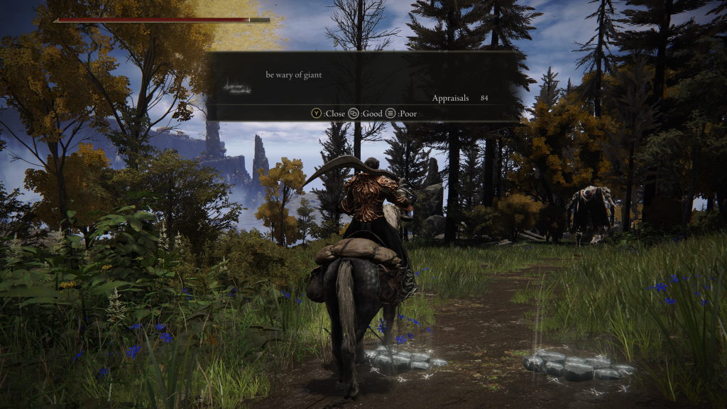
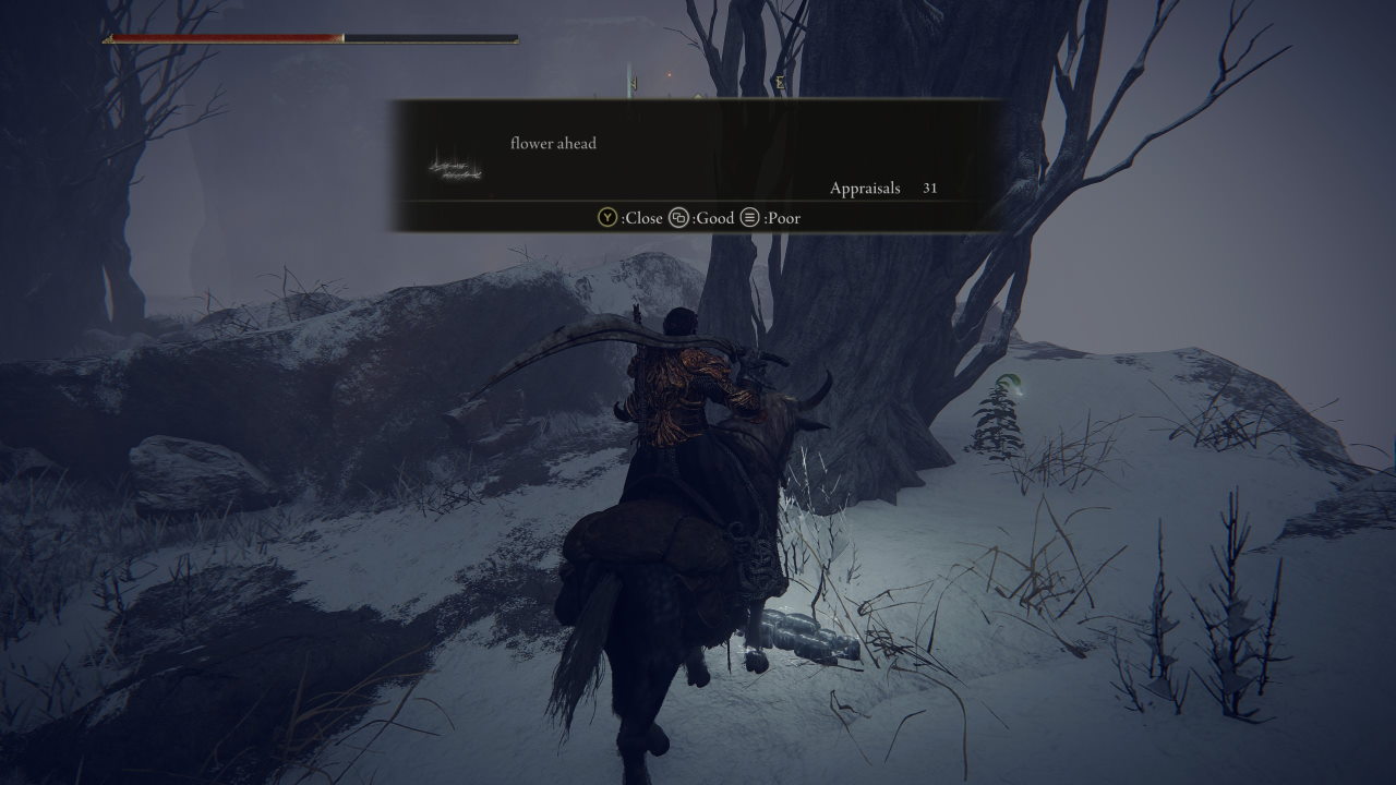
In Elden Ring players can create messages
given lists of words and templates, see some examples below

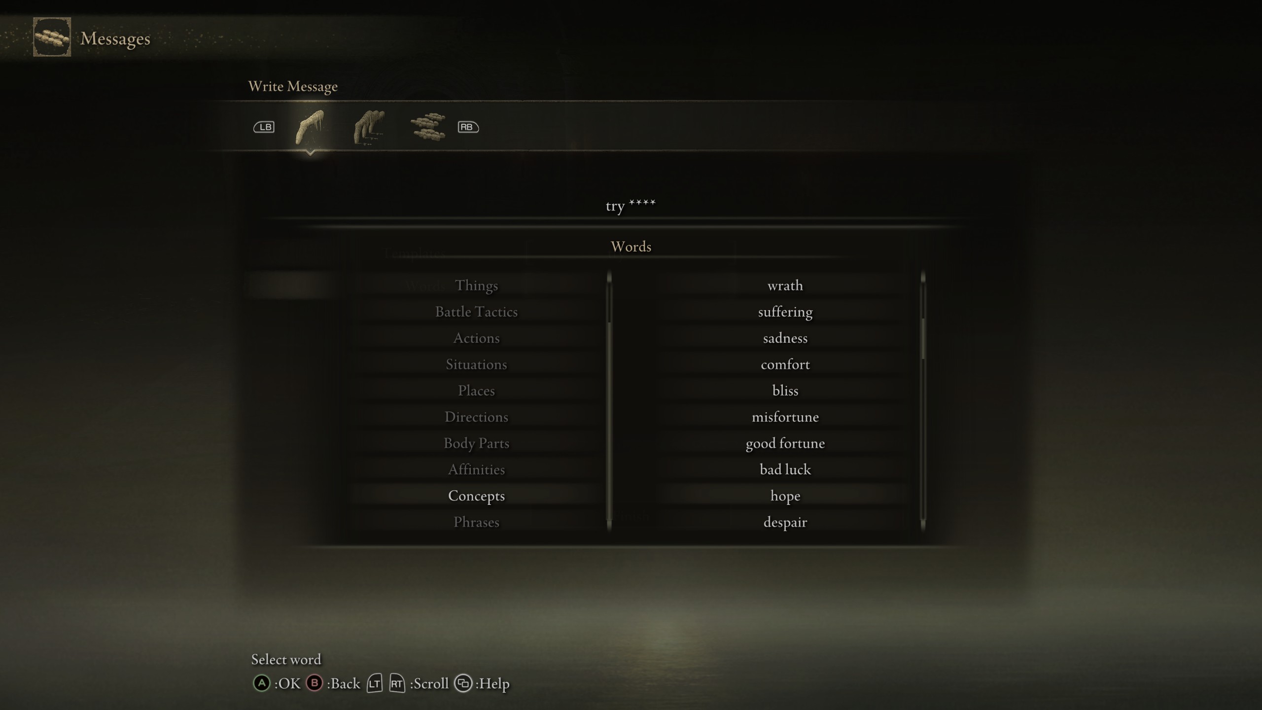
Messages often provide insight into the surrouding envirnment, though more often than not they are just someone being silly
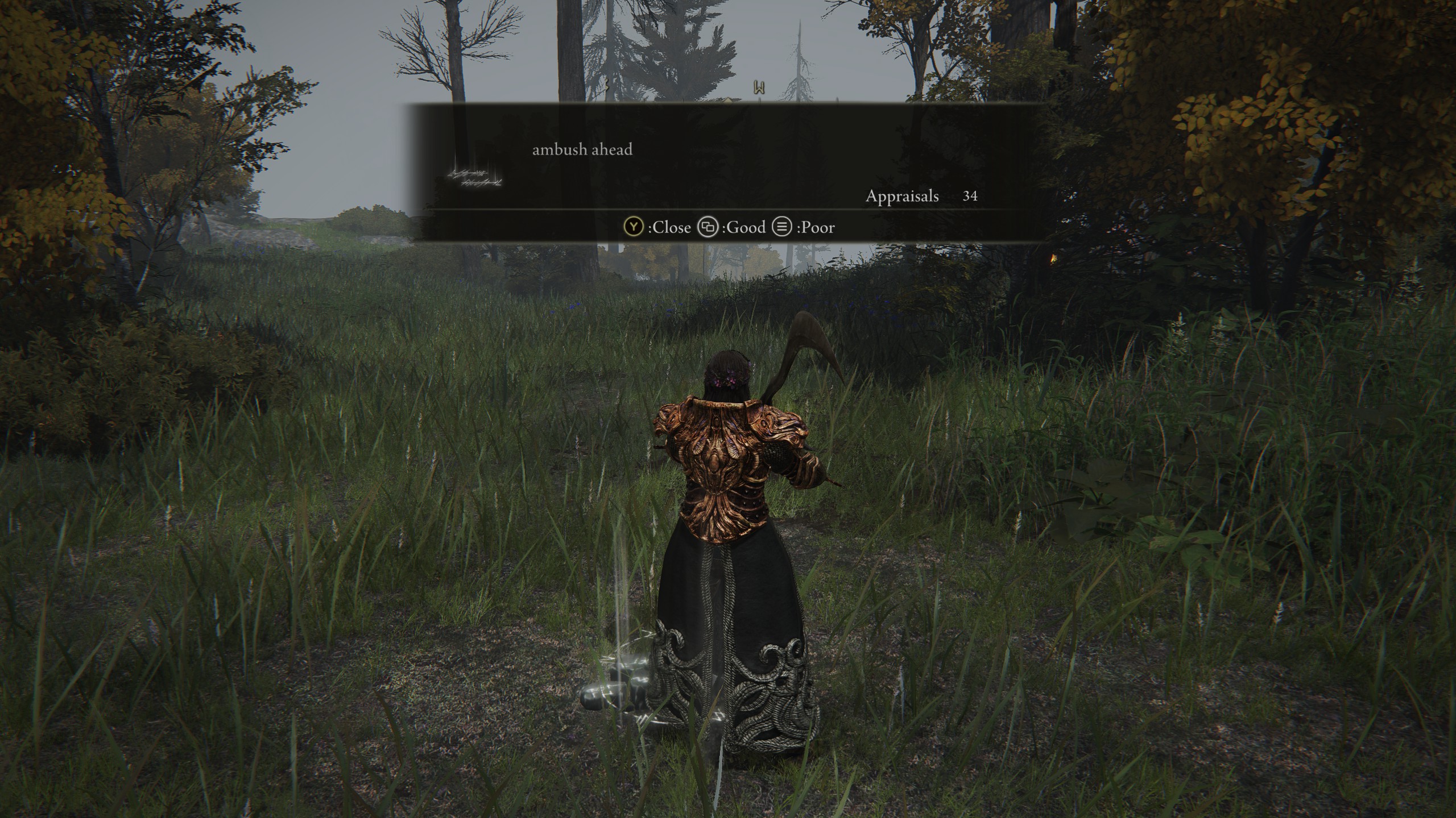
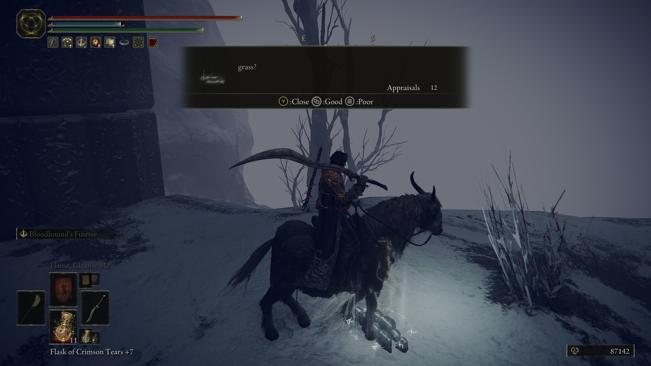
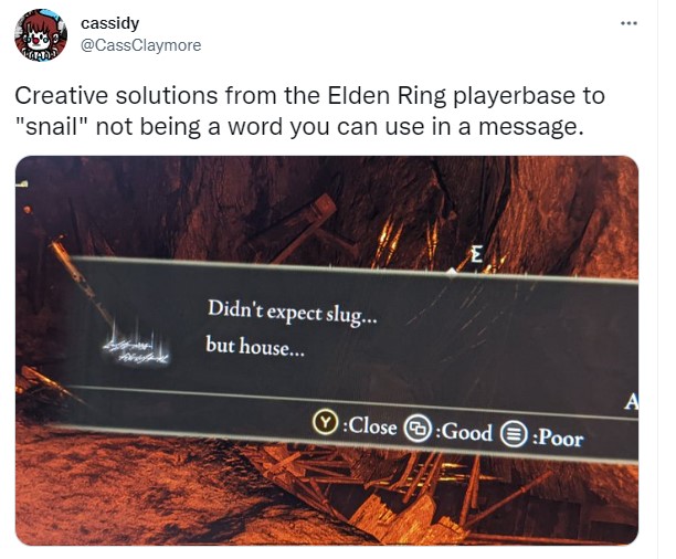
And sometimes they can make surprisingly clever use of the limited template system
If you arent an Elden Ring or Dark Souls fan don't worry I've also created examples with sentences from the Harry Potter books and of course with dialogue from the show Sailor Moon, the links are at the end of this article.
There are 368 words and 25 templates, so for single sentences in Elden Ring (without getting into combining two sentences with conjunctions) we have 368*25 = 9200 possible different sentences. The embeddings are created ahead of time and stored but when it's time to search that's 9200 arrays of 512 floats. To check the cosine similarity of one against all of them is not an outlandish task, especially when utilizing the gpu, but depending on the device running the search it can take upwards of a minute, checking the magnitude and dot product of vectors involves a lot of operations for vectors at higher dimensions.
Fortunately, there is a way to narrow our search results before
comparing the embeddings.
Locality Sensitive Hashes
Locality sensitive hashing involves generating random vectors with the same number of dimensions as our sentence embeddings and using them to divide the embeddings into groups or bins.
We divide embeddings into groups by checking if the dot product
between the randomly generated vector (or projection) and the
sentence embedding is positive or negative. Giving its hash a 1 or 0 respectively.
Remember vectors with an angular difference of more than 90°s will have a negative dot product,
and a positive dot product otherwise
Embeddings with different hashes are in different bins.
Let's look at one embedding, a, and one projection, p₁
Move them around to see how the hash for embedding a changes.
We can then use
multiple projections to group embeddings by the bins they are divided into, we will do this by again
giving the embeddings a 1 or
0 for a positive or negative dot product (within 90 or not) for each
projection. If an embedding is within 90° of the first projection (positive dot product)
we will add a 1 to its hash and then if it is not within 90 of the 2nd projection
(negative dot product) we add a 0 to its hash, and so on, the number of projections we have will
be our hash length since an embedding gets a 0 or 1 in its hash for
each projection.
Now let's look at two embeddings, a and b, and three projections p1,p2,p3
If two sentence embeddings(vectors) point in a similar direction, they are more likely to end up in
the same bin. If the vectors are 180° apart or have a cosine similarity
of -1, they will never be in the same bin, if they are 90° apart or have a
cosine sim of 0, there is a 50% chance they will be in the same bin,
and 100% chance if they are 0° and have cosine similarity of 1.
The formula for the probability of two vectors being in the same bin
would be 1-d/dc where d is the distance between the vectors and dc is
the max distance (d/dc is the probability they are in the same bin so 1-d/dc is the probability they
aren't)
We could use angular distance for this and see
1-90/180 = 0.5 or 50%. And could also normalize this to a max distance of 1 to view more easily on a
graph.
The probability of two events happening is (probability of event
1)X(probability of event 2)
Like rolling a 4 on a 6 sided dice twice in a row would be 1/6 X 1/6
So using the formula above 1-d/dc we can multiply it by itself for
the number of projections we have to see how the probability of two
embeddings being in the same bins based on their distance changes.
This would give us (1-d/dc)^k where k is the number of projections.
Increasing k reduces the chance of collision(two embeddings having
the same hash) since there are more opportunities for a projection
to divide them into separate bins.
With LSH the idea is that we have a good chance to end up with embeddings that are close to
eachother in the same bin,
though with only one hashtable there is a chance embeddings which are close could be divided by a
projection. We will look at multiple hashtables to deal with this soon.
Change the number of projections below to see how the probability of two embeddings being in the same bin based on their distance changes.
This will help us speed up searches by checking a new embedding (not
in our collection of sentences from Elden Ring, Harry Potter, or Sailor Moon) with
our projections and then only comparing it with embeddings that have
the same hash. We can adjust k to tune the probability of there
being a collision based on the distance between the embeddings.
Let's take a look at a rough python example we could use to create a hash table for our sentence tensors
hashtableLength = 5 #will also be our number of projections
inputArrayDims = 512
projections = []
hashTable = {}
#these are our previously generated sentence embeddings
with open('Tensors.json') as f:
    tensors = json.load(f)

#add an empty array to hold each projection
for i in range(hashtableLength):
	projections.append([])

#to each empty projection array add 512(same length as our tensors) random floats
for j in range(hashtableLength):
	for k in range(inputArrayDims):
		projections[j].append(np.random.randn())

#now projections is a 2d array of shape hashtableLength*imputArrayDims
#it is a set of made up projections/tensors/vectors, the same length as our sentence vectors

#for each tensor
for i, t in enumerate(tensors):
    #create an empty string to hold our hash
	hash = '';
	#then compare it to each projection in the hash table
	for k in range(hashtableLength):
	    #positive dot product(less than 90° distance) we add a '1'
		if(np.dot(t ,projections[k]) > 0):
			hash += '1'
		#and negative (greater than 90° distance) we add a '0'
		else:
			hash += '0'
	#if the hash string is already in our hash table,
	#add the index for this tensor to the list the hash points to
	if(hash in hashTable):
		hashTable[hash].append(i)
	#otherwise create an empty list with just that index to start
	else:
		hashTable[hash] = [i]
The 'hashTable' dictionary should now have each hash as a key and a list of the indices of the
tensors that have that hash, as the value.
We would then save the hashtable dict and our projections, and use them to generate a hash for a
search term,
then only check the cosine similarity of the search term tensor with the sentence tensors that have
the same hash,
we can get a list of those indices quickly since we have our hashtable dict.
Let's look at an example of this in javascript
apologies for hopping between languages but it's easy to write utility programs in python and
then obvs I
want this to be a web app so all the other stuff is js
//generated from python file
projections = [...]
hashTable = {}

sentences = ["","",...]
tensors = [[...],[...],...]

searchTerm = document.getElementById("searchTerm").value;
queryEmbedding = []
queryEmbedding.push((await model.embed(searchTerm)).unstack()[0])

//this need to match the length used in the python file
hashtableLength = 5;
inputArrayDims = 512;

hash = '';
//for each projection in the hashtable
for(j = 0; j < hashtableLength; j+= 1){
	//check the dot product of the search term embedding with the projection
	if(math.dot(queryEmbedding[0].arraySync(),projections[j]) > 0){
		//if positive(within 90°) hash gets a '1'
		hash += '1';
	}
	//otherwise if negative(not within 90°) hash gets a '0'
	else{
		hash += '0';
	}
}

//now we have built the hash for query embedding by running it through the same projections
//we ran all the sentence embeddings through to create our hash table,
//we can now use the hash to check our hash table for the indices that have the same hash!

indicesToCompare = [];

//there is a chance our search term dosen't share its hash with any of the tensors so we check the hash exists
if(hash in hashTables[i]){
	indicesToCompare = hashTable[hash];
}

//check cosine similarity for each tensor that had the same hash
scores = new Array(tensors.length).fill(1);
for(i = 0; i < indicesToCompare.length; i+= 1){
    score = tf.losses.cosineDistance(tensors[indicesToCompare[i]], queryEmbedding[0], 0);
    scores[indicesToCompare[i]] = score.arraySync();
}
We will then have the 'scores' array which has the cosine similarity for each of the tensors from the indices to compare list, and the rest that we didn't compare will be a 1. We can sort these values to find the sentence tensors that are closest to our search term.
We can also create multiple hash tables to increase the chance of
collision, since just one will give us a high chance of false
negatives, since even if two vectors have a fairly high angular similarity there is still a chance
for one of the projections to divide them, with several hashes
there is a much better chance that vectors that have higher angular similarity will have a bin
collision in at least one hash table.
Take a look at the chart above and adjust the number of projections
to 5,
This gives us a good chance to not have a collision for embeddings with a distance greater than 0.6,
but ideally we would like to see the line shoot up more quickly after that, since at a distance of
0.2 which
is quite close there is still only slightly better than a 25% chance we will have a collision.
We will be able to fix this with multiple hash tables.
So looking at our formula, (1-d/dc)^k is
our probability of collision (Pc) right now for one hash of length k,
1-Pc is the probability that we don't have a collision for a hash,
(1-pc)^L is the probability we don't have a collision for L number of
hashes, and finally 1-(1-pc)^L is the probability we do have a
collision, so thats 1-(1-(1-d/dc)^k)^L
at least, that is my understanding of how the probability works out and I get the same looking graph
as in this paper:
see page 1116.
visualizing this below helps us get a good idea for
probability based on distance, hash length, and number of hashes. Here is a a youtube video I managed to find while trying to understand all of this as well!
If we were to go with 20 projections and 2000 hash tables we are pretty much guaranteed to have collisions for hashes with a distance less than 0.25, but the trade off is the information for that many hash tables would take up a huge amount of space, so we still want to look for that trade off between accuracy and performance.
Now let's look at some code examples similar to the ones above but adjusted to use multuple hash
tables
first the python code to create the hash tables and projections.
numberOfHashtables = 16
hashtableLength = 5
inputArrayDims = 512
projections = []
hashTables = []

for i in range(numberOfHashtables):
    hashTables.append({})

for i in range(numberOfHashtables):
    projections.append([])
    for j in range(hashtableLength):
        projections[i].append([])

for i in range(numberOfHashtables):
    for j in range(hashtableLength):
        for k in range(inputArrayDims):
            projections[i][j].append(np.random.randn())


with open('Tensors.json') as f:
    tensors = json.load(f)

for i, t in enumerate(tensors):
    for j in range(numberOfHashtables):
        hash = '';
        for k in range(hashtableLength):
            if(np.dot(t ,projections[j][k]) >0):
                hash += '1'
            else:
                hash += '0'
        if(hash in hashTables[j]):
            hashTables[j][hash].append(i)
        else:
            hashTables[j][hash] = [i]
and the javascript
//generated from python file
projections = [...]
hashTables = {}

sentences = ["","",...]
tensors = [[...],[...],...]

searchTerm = document.getElementById("searchTerm").value;
queryEmbedding = []
queryEmbedding.push((await model.embed(searchTerm)).unstack()[0])

//these need to match the lenths used when generating the number
//of hash tables and length
numberOfHashtables = 16;
hashtableLength = 5;

inputArrayDims = 512;

queryHashes = [];
for(i = 0; i < numberOfHashtables; i+= 1){
    hash = '';
    for(j = 0; j < hashtableLength; j+= 1){
        if(math.dot(queryEmbedding[0].arraySync(),projections[i][j]) >0){
            hash += '1';
        }
        else{
            hash += '0';
        }
    }
    queryHashes.push(hash);
}

indicesToCompare = [];
for(i = 0; i < queryHashes.length; i+= 1){
    if(queryHashes[i] in hashTables[i]){
        indicesToCompare.push(...hashTables[i][queryHashes[i]]);
    }
}

//turn the list into a set to remove duplicates
indicesToCompare = [...new Set(indicesToCompare)];

scores = new Array(tensors.length).fill(1);
for(i = 0; i < indicesToCompare.length; i+= 1){
    score = tf.losses.cosineDistance(tensors[indicesToCompare[i]], queryEmbedding[0], 0);
    scores[indicesToCompare[i]] = score.arraySync();
}
I'll include all the full code that I used on this projects github page
So as we increase the number of hash tables we have more chances for
embeddings to fall into the same bin at least once, and embeddings
that are close are likely to fall into the same bin even more
often.
This leads us to a final bit of optimization, we can
increase the number hash tables and use the frequency of
bin collision as our similarity score to remove the need for
checking cosine similarity entirely, this also eliminates the need
to store the sentence embeddings to compare, we only need to create
an embedding for the search term and create hashes of it by checking
it with our projections for each hash table.
projections = [...]
hashTables = {}

sentences = ["","",...]

searchTerm = document.getElementById("searchTerm").value;
queryEmbedding = []
queryEmbedding.push((await model.embed(searchTerm)).unstack()[0])


numberOfHashtables = 300;
hashtableLength = 5;
inputArrayDims = 512;


queryHashes = [];
for(i = 0; i < numberOfHashtables; i+= 1){
    hash = '';
    for(j = 0; j < hashtableLength; j+= 1){
        if(math.dot(queryEmbedding[0].arraySync(),projections[i][j]) >0){
            hash += '1';
        }
        else{
            hash += '0';
        }
    }
    queryHashes.push(hash);
}

//we run the query through each hashtable and get the indices of the embeddings that it collides with
//if two embeddings are very close they could collide for every hash table, then we would see them 500 times in indices to compare
//or if two embeddings are very far apart we probably wont see them in the list at all
indicesToCompare = [];
for(i = 0; i < queryHashes.length; i+= 1){
    if(queryHashes[i] in hashTables[i]){
        indicesToCompare.push(...hashTables[i][queryHashes[i]]);
    }
}


//this snazzy bit of js will take the indicies to compare list and return a dictionary called map
//with each index that occured at least once as the key and the number of occurances as the value
var map = indicesToCompare.reduce(function(p, c) {
  p[c] = (p[c] || 0) + 1;
  return p;
}, {});

//this will take that dictionary and sort the keys(the indices of the embeddings)
// by the values(the number of times that embedding collided with our query hash in our hashtables)
var results = Object.keys(map).sort(function(a, b) {
  return map[b] - map[a];
});

//so now the results list is a list of the indeices of the sentence embeddings sorted descending by
//the number of collisions they had with the query embedding, so sorted from best match going down
//we can reference those indices back to our sentences list to display them

res = ""
table = document.getElementById("results");
table.innerHTML = "";
for(var i = 500; i >= 0; i-= 1){
 var row = table.insertRow(0);
  var cell1 = row.insertCell(0);

  cell1.innerHTML = sentences[results[i]];

}
This will result in a loss of accuracy
since collision is probability based as we saw above, but with enough
tables we can achieve decent results, especially for
something as subjective as comparing sentences. Less disk space is
needed and search time is further improved. I don't have a fantastic way to decide what values to
use to achieve that but for but from looking at the charts and trying things out I've found around
200-300 hashtables
with a length of 5 each produces good search results for searching with hashes only, for my sentence
sets.
Another way to understand this idea of scoring results by hash collisions only is to first take a look back at this chart
and change the number of projections(length of each hash table) to 5, and the number of hash tables to 1
Take a look at the curve formed showing the probability of getting one match with our one hash table.
Then change the number of hash tables to 100, this curve shows the probability of getting at least one match, but we could get up to 100, you can think of it as stacking the probability of the last curve 100 times.
For this last method of scoring by just checking frequency of bin/hashtable collision as our similarity score, we are just checking the 100 randomly generated hashtables,
each one with the probability you saw for the first curve (5 projections 1 table)
and adding up how many times we get a hash collision as our score.
If you're curious about this blog or still dont fully understand, feel free to shoot me an email at colourofloosemetal@gmail.com, I would be happy to chat about this project.
I havent talked too much about the actual universal sentence encoder model since it isn't really the main topic of this article, but it is worth mentioning that all the examples use the "lite" version of the model which is many many times smaller than the main version, this is to allow it to run in your browser. In the future I might try to run the larger model locally to see how the results improve. The lite version still gives excellent results but it probably wont pick up on things like idioms and is more likely to interpret text literally if you try some.
Live Demos
Do Not try to search before the loading message goes away, if the loading message seems like it is taking an absurdly long time to go away try the example on desktop or refresh the page
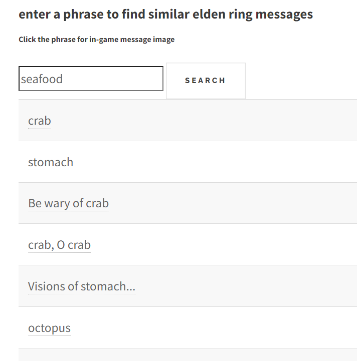
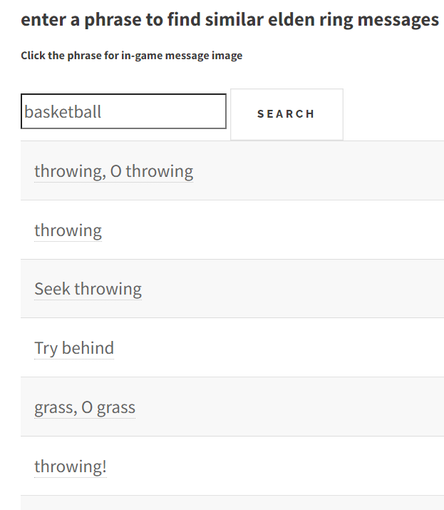
Elden Ring Messages
If you've played elden ring this is fantastic for finding messages, but with less than 10k messages to search from the results can be lacking
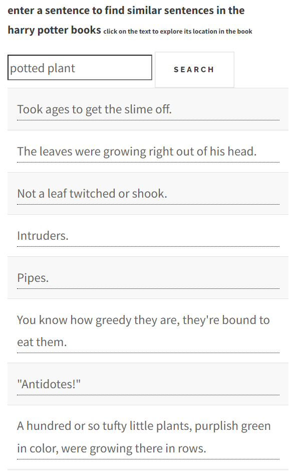
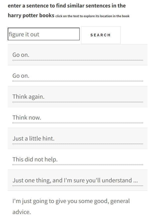
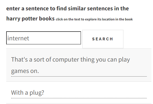
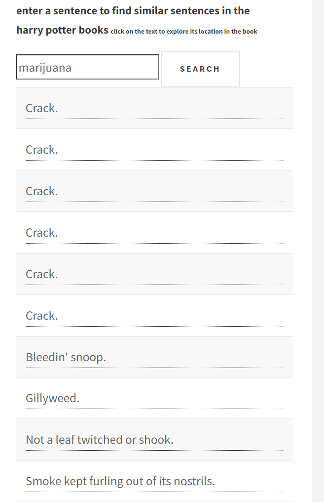
Harry Potter bookswith close to 10x the results of the elden ring messages there are some interesting sentence to be found
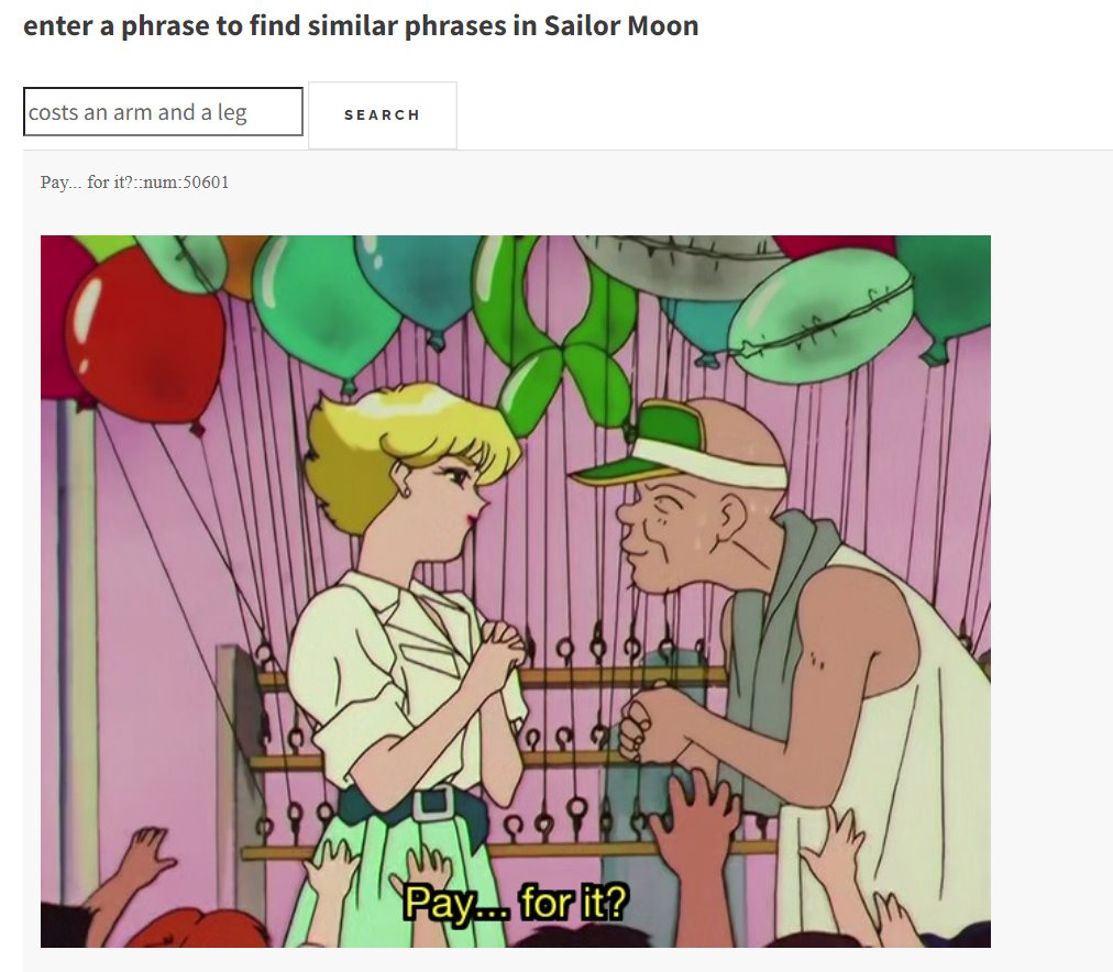
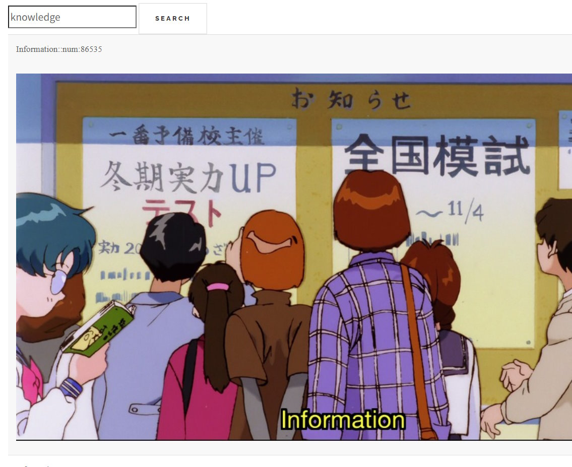
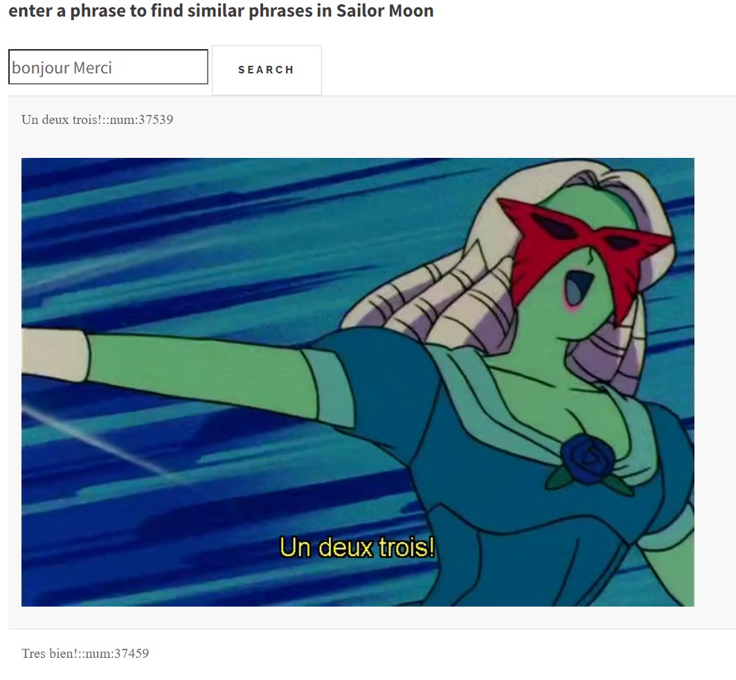
Sailor Moon
💯
here are some interestng results from each searcher
Starting with Elden Ring
Harry Potter
And of course Sailor Moon


please also email me screenshots like these if you get any fun results colourofloosemetal@gmail.com